2.6. Evaluations
What is an evaluation?
Model evaluation is a fundamental step in the machine learning workflow that involves assessing a model's predictions to ensure its reliability and accuracy before deployment. It acts as a quality assurance mechanism, providing insights into the model's performance through various means such as error metrics, graphical representations (like validation curves), and more. This step is crucial for verifying that the model performs as expected and is suitable for real-world applications.
Why should you evaluate your pipeline?
Machine learning models can sometimes behave in unpredictable ways due to their inherent complexity. By evaluating your training pipeline, you can uncover issues like data leakage, which undermines the model's ability to generalize to unseen data. Rigorous evaluation builds trust and credibility, ensuring that the model's performance is genuinely robust and not just a result of overfitting or other biases.
For more insights on data leakage, explore this link: Data Leakage in Machine Learning.
How can you generate predictions with your pipeline?
To generate predictions using your machine learning pipeline, employ the hold-out dataset (test set). This approach ensures that the predictions are made on data that the model has not seen during training, providing a fair assessment of its generalization capability. Here's how you can do it:
# Generate predictions
predictions = pd.Series(final.predict(inputs_test), index=inputs_test.index)
print(predictions.shape)
predictions.head()
Also, leverage the insights from your hyperparameter tuning process to understand the effectiveness of various configurations:
# Analyze hyperparameter tuning results
results = pd.DataFrame(search.cv_results_)
results = results.sort_values(by="rank_test_score")
results.head()
What do you need to evaluate in your pipeline?
Evaluating your training pipeline encompasses several key areas:
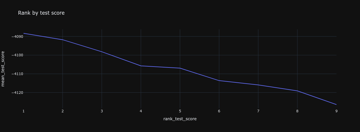
Ranks
When analyzing the outcomes of hyperparameter tuning, focus on:
- Identifying ineffective hyperparameter combinations to eliminate.
- Determining if the best hyperparameters are outliers or represent a common trend.
This helps in deciding whether to expand or narrow the search space for optimal parameters.
Example:
# Visualize rank by test score
px.line(results, x="rank_test_score", y="mean_test_score", title="Rank by test score")
Params
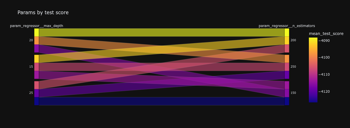
Investigate which hyperparameters lead to better performance by:
- Spotting trends that suggest optimal settings.
- Identifying hyperparameters with minimal impact, which could be omitted.
This enables pinpointing the most effective hyperparameters for your specific problem.
Example:
# Visualize hyperparameter impact
dimensions = [col for col in results.columns if col.startswith("param_")]
px.parallel_categories(results, dimensions=dimensions, color="mean_test_score", title="Params by test score")
Predictions
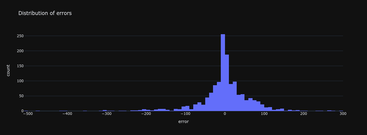
Compare predictions with observed outcomes on the untouched test period and a baseline. Similar marginal distributions alone do not establish good predictions.
Example with a single metric:
from sklearn import metrics

# Calculate a performance metric
observed = targets_test.astype("float64")
predicted = predictions.astype("float64")
score = metrics.mean_squared_error(observed, predicted)
errors = pd.DataFrame({"error": observed - predicted})
score
Convert unsigned counts before computing residuals or metrics. Otherwise an overprediction can wrap a negative residual into a large positive number; the reference package makes this conversion at its metric boundary while keeping count schemas unchanged.
Example with a distribution:
# Visualize distribution of errors
px.histogram(errors, x="error", title="Distribution of errors")
Feature Importances
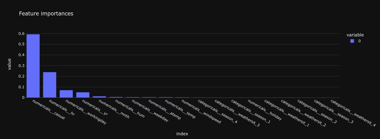
Understanding which features most significantly influence your model's predictions can streamline the model by removing non-essential features. This analysis is more straightforward in models based on linear and tree structures.
Example:
# Determine feature importances
importances = pd.Series(
    final.named_steps["regressor"].feature_importances_,
    index=final[:-1].get_feature_names_out(),
).sort_values(ascending=False)
print(importances.shape)
importances.head()
How can you ensure your pipeline was trained on enough data?
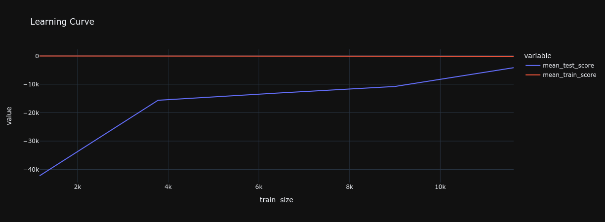
Employing a learning curve analysis helps you understand the relationship between the amount of training data and model performance. Continue adding diverse data until the model's performance stabilizes, indicating an optimal data volume has been reached.
Example using scikit-learn's learning curve:
# Analyze learning curve
train_size, train_scores, test_scores = model_selection.learning_curve(
    final, inputs_train, targets_train, cv=splitter, scoring=SCORING, random_state=RANDOM,
)
learning = pd.DataFrame(
    {
        "train_size": train_size,
        "mean_test_score": test_scores.mean(axis=1),
        "mean_train_score": train_scores.mean(axis=1),
    }
)
px.line(learning, x="train_size", y=["mean_test_score", "mean_train_score"], title="Learning Curve")
How can you ensure your pipeline captures the right level of complexity?
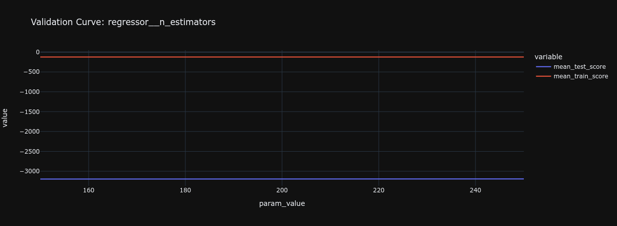
To balance complexity and performance, use validation curves to see how changes in a model parameter (like depth) affect its performance. Adjust complexity to improve performance without causing overfitting.
Example with scikit-learn's validation curve:
# Explore validation curves for different parameters
for param_name, param_range in PARAM_GRID.items():
    print(f"Validation Curve for: {param_name} -> {param_range}")
    train_scores, test_scores = model_selection.validation_curve(
        final, inputs_train, targets_train, cv=splitter, scoring=SCORING,
        param_name=param_name, param_range=param_range,
    )
    validation = pd.DataFrame(
        {
            "param_value": param_range,
            "mean_test_score": test_scores.mean(axis=1),
            "mean_train_score": train_scores.mean(axis=1),
        }
    )
    px.line(
        validation, x="param_value", y=["mean_test_score", "mean_train_score"], title=f"Validation Curve: {param_name}"
    )
Practice: an untouched future batch
Goal: tune on past observations, compare the selected model with a simple baseline, and keep the newest 24 observations out of every tuning fold. Start in the course repository with the pinned toolchain installed; the synthetic data needs no download.
Before running, predict whether a mean-only baseline can extrapolate an increasing trend. Then run:
uv run --locked examples/temporal_evaluation.py
The script below is the source executed by the course gate:
# /// script
# requires-python = ">=3.14"
# dependencies = ["numpy>=2.1.3", "scikit-learn>=1.9.0"]
# ///
"""Tune on past observations and evaluate once on the untouched future."""

import numpy as np
from sklearn.dummy import DummyRegressor
from sklearn.linear_model import Ridge
from sklearn.metrics import mean_squared_error
from sklearn.model_selection import GridSearchCV, TimeSeriesSplit
from sklearn.pipeline import make_pipeline
from sklearn.preprocessing import StandardScaler

# Synthetic time-ordered observations: no downloads or external services.
time = np.arange(120, dtype=float).reshape(-1, 1)
demand = 20 + 3 * time.ravel() + np.sin(time.ravel())
boundary = 96
inputs_train, inputs_test = time[:boundary], time[boundary:]
targets_train, targets_test = demand[:boundary], demand[boundary:]
assert inputs_train.max() < inputs_test.min()
cv = TimeSeriesSplit(n_splits=3)
for train, validation in cv.split(inputs_train):
    assert train.max() < validation.min()
    assert inputs_train[train].max() < inputs_train[validation].min()
    assert validation.max() < boundary

# Each fold fits its own scaler. The final refit sees only the training period.
search = GridSearchCV(
    make_pipeline(StandardScaler(), Ridge()),
    {"ridge__alpha": [0.01, 0.1, 1.0]},
    scoring="neg_mean_squared_error",
    cv=cv,
    n_jobs=1,
)
search.fit(inputs_train, targets_train)
np.testing.assert_allclose(search.best_estimator_["standardscaler"].mean_, inputs_train.mean(axis=0))

# Fix the selected model before looking at holdout results.
baseline = DummyRegressor(strategy="mean").fit(inputs_train, targets_train)
model_mse = mean_squared_error(targets_test, search.predict(inputs_test))
baseline_mse = mean_squared_error(targets_test, baseline.predict(inputs_test))
assert model_mse < baseline_mse
print(f"Chronology and train-only preprocessing passed; model MSE={model_mse:.3f}, baseline MSE={baseline_mse:.3f}.")
Verify: the command prints that chronology and train-only preprocessing passed, followed by the two measured MSE values. This synthetic result demonstrates the evaluation procedure; it does not establish bike-demand performance. Afterward, the repository still contains the lab and its dependency lockfile; no datasets or models were saved.
Investigate: temporarily reverse the row order before splitting. Which assertion should fail, and why would ignoring row order make the evaluation misleading? Restore the lab before running mise run test again.